Evaluating metadata classification
My last post covered how I evaluated chunking for FindFiles, a local-first document search tool: starting from a baseline of 1,000-character chunks with 200 characters of overlap, I tested against a labeled set and — to my surprise — found that smaller chunks retrieved noticeably better.
Better chunking improved retrieval; the system pulled up the right documents more often. But retrieving the right document is only half the job. Before the tool can decide whether a document satisfies a task, it has to recognize what the document actually is — and that recognition step was getting it wrong. Improving retrieval had simply exposed the next constraint: classification.
Where the pipeline stands
FindFiles takes a task — say, filing taxes — and reports which of the required documents are present in a folder and which are missing. Two stages produce that report:
- Retrieval — find the documents relevant to the task.
- Classification — at index time, a local model reads each document and tags it with metadata: what type it is (W-2, lease, passport), its date, who issued it.
Retrieval decides which documents get considered. Classification decides what those documents are. The gap report needs both to be right; the chunking work addressed the first, and the second is still unreliable.
The classification bottleneck
Retrieval finds the right candidates now. The report still gets things wrong, and the reason is the other stage.
Gap detection uses the document type and date to decide whether a retrieved candidate is actually the document the task needs. Those labels come from a local model reading each file — and they’re wrong more often than they’re right. I measured it: llama3.2, a 3-billion-parameter model, picks the correct type from a fixed list 22.6% of the time — 12 of 53 documents. It isn’t even consistent between runs; the same medical claim form came back as “W-2” once and “bank statement” the next time.
The consequence is direct. If the metadata the final answer depends on is wrong more often than not, the report can’t be trusted without checking every entry by hand — which defeats the purpose of the tool. Classification is where the next stretch of work has to go.
The evaluation plan
The plan mirrors the chunking work, because it worked there: a small labeled test, honest metrics, and one variable changed at a time, so a gain can be traced to a specific cause instead of a guess about which of several changes helped.
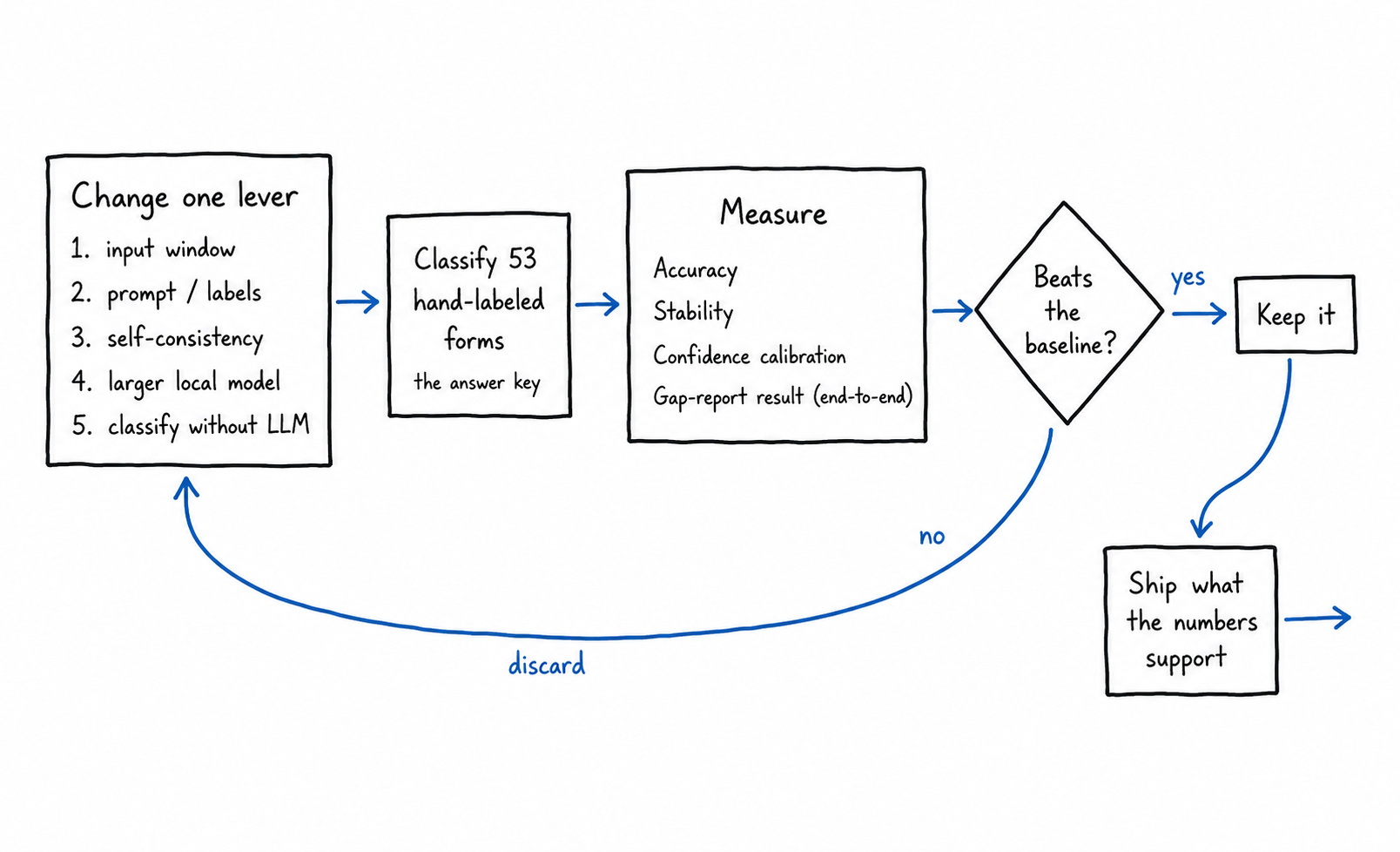
The ground truth. I hand-labeled those same 53 real government forms with their correct type, date, and issuer. That’s the answer key to score the model against.
What to measure. Raw accuracy is the obvious metric, but not enough on its own:
- Accuracy — does the predicted type and date match the label?
- Stability — ask the model the same question several times; does it give the same answer? An unstable classifier is a problem even when it’s sometimes right.
- Confidence calibration — the model reports a confidence score with each label. The system already treats low-confidence labels with more caution, so that score has to actually track correctness. If a confident label is wrong as often as an unsure one, the score is noise and the caution built on it does nothing.
- The end-to-end effect — does a more accurate classifier actually produce a better gap report? Field accuracy is a proxy; the report is the product. So every change is measured against the report, not only against the labels.
What to tune. The levers most likely to move the number, ordered from least to most effort:
- Input window — how much of the document the model reads, and which part. These forms put the title at the top but the date and issuer further down, so reading only the first stretch of text can miss what matters.
- The prompt and label set — giving the model a few worked examples, or a shorter, clearer list of types to choose from. A small model may do better with a coarser set of labels it can actually tell apart.
- Self-consistency — run the model several times and take the majority label. This addresses the instability directly instead of hoping a single run lands right.
- A larger local model — still on your machine and private, but with more capacity than a 3B model. Likely the biggest single lever, and the slowest to run, so it comes after the lighter changes.
- Classifying without the LLM — since retrieval already works well, I can label a new document by comparing it to the ones I’ve already labeled: find the most similar labeled documents by embedding and borrow their label. If an unknown form’s nearest neighbors are all W-2s, call it a W-2. It’s worth checking whether that beats asking a 3B model to name the type from scratch.
The order is the same as before: get a baseline, run the lighter changes, then the heavier ones, and ship only what the numbers support.
Committing to the plan before the results
I’m publishing the plan now, before there’s a single new number, on purpose. Fixing the definition of “better” — and committing to measure it against the gap report, not just the labels — before any experiment runs keeps me from quietly redefining success once the results arrive. The numbers will be their own post. This one sets the starting point: classification is the current bottleneck, the target is defined, and the plan is in place.